Gridded datasets take point measurements of climate variables and then combines them in one of the following ways:

1. Averaging climate values or anomolies of the stations located within a grid’s cell
2. Interpolation of climate or anomolies, which is based on the distance between the stations the values are collected from
3. Interpolation that not only is based on distance, like the prior, but also is based on topography.

These datasets are primarily used for precipitation, surface temperature, and sea surface temperature.

Check ’em out >> datasets at the National Center for Atmospheric Research (NCAR)

It seems like everyone’s got their own version of a gridded dataset. The Hadley Centre in the UK created HadAT2  and QUARC, the National Oceanic and Atmospheric Administration (NOAA) created RATPAC, and even the University of South Wales’  Steven Sherwood developed the Iterative Universal Kriging (IUK) dataset in Australia. You can find a (incomplete) list of additional gridded datasets in Winkler et al. 2011.

But where do these climate measurements come from?

We’re using radiosondes, satellites, and ground based remote sensing to collect a variety of measurements. To truly understand climate, we need not only long-term data but large spatial representation.

 

Now, consider the many layers in the atmosphere. We want to make sure our data samples at the right height! Notice how altitude and temperature are related depending on the layer in the atmosphere in the image below (thanks National Weather Service)

• Troposphere: Where weather occurs
• Stratosphere: Temperature remains constant until it reaches the upper area of this layer, where the ozone concentration is. The effect of the ozone absorbing ultraviolet radiation causes this region to be warmer.
• Mesosphere: Temperature decreases as height increases.
• Thermosphere: Temperature increases due to UV radiation absorption by oxygen and nitrogen. Temperature is high and density is low, so gasses don’t retain much heat.

The distinct changes between the layers can tell us a lot about the changes in climate, specifically relating to carbon!

 

Measuring Upper Atmospheric Variables

Radiosondes, satellites, and remote sensing, oh my.

 

Radiosonde and rawinsondes

These measure the troposphere and the lower stratosphere. The instruments are attached to balloons and use radio communication to relay real time data back to Earth. Apart from a parachute and GPS, they include:

• Aneroid barmeter (measures pressure)
• Thermistor (measures temperature)
• Hygristor (measures relative humidity)

Many errors come with radiosonde data. First of all, they drift away after release and can travel as far as 200km from the original testing site!

Release in the U.S. occurs twice a day at ~92 stations, but there are about 1,000 stations around the globe. This creates a second cause for error, there are different practices in implementing the method as well as an uneven spatial distribution.

Additional worries include changes in:

• sensor types
• signal processing algorithms
• instrument calibration procedures
• reporting and coding practices
• archiving procedures

Overall, data is again affected by changing procedures, sensors, failed equipment and the chances of this happening at multiple stations— with some even unaware of it. This can seriously effect the long term changes we want to study.

Gridded Datasets for Radiosonde

HadAT2 | Hadley Centre, UK

One of the first developed gridded, upper-air data sets. It studies 10-5 degrees latitude and is composed of 676 individual radiosonde stations with long-term records. Temperature was averaged in each grid cell. This dataset was last updated 2012.

 

QUARC | Hadley Centre, UK

QUARC, known for Quantifying Uncertainty in Adjusted Radiosonde Climate records, is another temperature ensemble based on methodological decisions (unlike HadAT2, which was based on long-term record). This dataset detects the bias and uncertainty found in HadAT2 data using the Nearest Neighbor Average.

 

RATPAC | NOAA, US

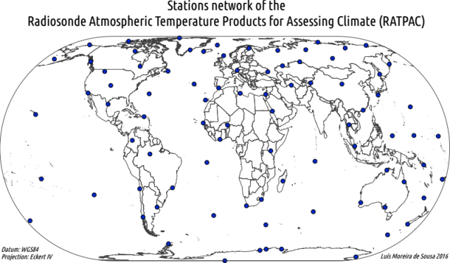
The Radiosonde Atmospheric Temperature Products for Assessing Climate was developed in the early 2000s to detect the time series of temperature anomalies. This is a global sample with 87 stations and comes highly recommended for assessing long-term changes in temperatures for the troposphere and lower stratosphere. The result has created RATPAC-A and RATPAC-B.

RATPAC-A

RATPAC-A contains adjusted global, hemispheric, tropical, and extratropical mean temperature anomalies.” Data was collected from two sources: 1958-1995 spatial averages of the Lanzante et al. (2003a,b; hereafter LKS) adjusted 87-station temperature data; after 1995, the Integrated Global Radiosonde Archive (IGRA) station data was used. The “first difference method” combined the IGRA data to reduce the influence that inhomogeneities had. RATPAC-A is used for analyses of interannual and longer-term changes in global, hemispheric, and tropical means. (source: NCDC)

 

IUK |University of South Wales, Australia; Steven Sherwood

Reports the temperature and wind shear at mandatory reporting levels dating to 1959-2015. This includes 527 radiosonde stations, which are divided into two groups A and B. Group A has substantial data recorded twice a day, while Group B has fewer data but has stations located in the tropics and southern hemisphere). Group A is more reliable. Even so, biases remain in the dataset such as cooling in the tropics.

 

 

Gridded Datasets for Satellites

First, a little history

Satellite observations for temperature first began around 1979. Satellites are able to measure climate variables as they collect or transmit radiation from a specified range on the electromagnetic spectrum. The “raw” data is then transposed by an algorithm into usable data.

Again, error can be introduced by these algorithms. Measurements taken at the point of interest, called in situ, are used to help adjust the observations.

There are two major types of satellites:

Geostationary

Geostationary operational environmental satellites (GOES) are used primarily for short-range sensing aka “nowcasting”. They are at high altitudes, 22,282 miles above the Earth, and rotate with the planet to concentrate on one area. The are directly above the equator and their locations vary by longitude only. The downfalls of geostationary satellites include low resolution of ground data since such a large area is detected, and the polar regions are not observed.

There is a worldwide network of satellites that cover the entire planet, including:

• GOES, US
• Meteosat, European Space Agency
• EUMETSAT, European Weather Satellite Organization
• GMS, Japan
• INSAT, India

 

Polar orbiting

Low earth range satellites are particularly important for climate monitoring. They rest above the earth at 400-1600 miles and revolve around. Since they are closer to Earth’s surface, they have a higher resolution. They also are not stationary and rotate over the Earth’s poles; their flight path is unlimited and they are able to observe places twice a day. Their sun-synchronous orbit allows them to view different latitudes at generally similar lighting conditions, as the local solar time is essentially unchanged.

Another worldwide network exists to cover as much of the planet as possible, including satellites from:

• Department of Defense, US DOD
• NOAA (soon to launch the JPSS series in 2017)
• EUMETSAT, Europe

 

Polar orbiting satellites are best used for climate studies. They measure long-term observations such as the land surface, biosphere, atmosphere and ocean. The drawbacks of satellites include time-varying biases, including:

• diurnal drift: over time the satellites drift away from their sun synchronous orbit
• orbital decay: the atmosphere itself will change over time due to variations in solar activity, this causes frictional drag on the satellite or even the geometry of the satellites view to become less accurate.
• inter-satellite biases
• calibration changes: due to heating and cooling of the instrument in space or from the launch

 

 

Resources:
Winkler, J. A., et al,. 2011. Climate scenario development and applications for local/regional climate change impact assessments: An overview for the non-climate scientist. Part II: Considerations when using climate change scenarios. Geography Compass, 5/6, 301-328.