ABSTRACT (Poster P-04) | Now published in Landscape Ecology rdcu.be/c9MHO

This study evaluated the contributions of land cover and land use change (LCLUC) and land management to landscape carbon production through a complex cause-effect path analysis of socioecological latent variables. Socioecological contributions to landscape carbon production are essential in landscape analysis, as their processes are both independent and interactive. We quantify the coherencies of social, economic and ecological variables and their impact on net primary production (NPP) in an agroecosystem. We ask whether LCLUC contributed to increased NPP and if land management and LCLUC play a more significant role than abiotic stressors on NPP. We applied a socioecological system framework to evaluate socioecological processes in the Kalamazoo River Watershed agroecosystem in southwest Michigan, USA from 1987 to 2017. Structural composition and functional contribution to NPP were evaluated by land cover type. We synthesized remote sensing, gridded climate, social and biophysical data, in a principle component analysis (PCA) to inform a partial least squares structural equation model (PLS-SEM). Land cover type contributes to anthropogenic processes, where cropland contributed to Land Management, forest and water to Land Cover Change, and urban land cover to Rural Development construct. Anthropogenic activities contributed more to NPP than abiotic processes. Attitudes of environmental stewardship strongly related to land use change likelihood. We disentangled contributions of anthropogenic and climatic changes in terrestrial carbon production and the societal ties to ecosystem health and potential carbon sequestration. No single landscape metric is suitable for all study areas; however, this framework is useful for landscape scale analysis of socioecological processes.

In plain language: What are the relationships and their strengths between human activities, ecosystem carbon production, and landscape composition?

These collectively shape the landscape’s carbon production, amongst other ecosystem health and functions like water and energy cycles. All these activities and functions can feel like Everything, everywhere, all at once, so we took bite-sized rates of their occurrence across time and space and modeled them in a structural equation model (SEM).

In this post, I’ll share my poster presentation from the 2023 International Association of Landscape Ecology North America Chapter (IALE-NA) Annual Meeting, March 20-23,. 2023.

The complexity and interactions between people and the environment and space and time can be overwhelming! The best way I can think about it is like the 2022 hit Everything, everywhere, all at once where the relationships and things we know have hidden layers of complexity across many levels.

How can we evaluate these socioecological relationships, then?

We selected the Kalamazoo Watershed in southwest Michigan, USA for our case study. The area is an agroecosystem, meaning that it’s largely centered around agriculture and therefore its ecologically and socially impacted (e.g., biodiversity may decrease, it’s frequently using chemicals, etc.). The Kalamazoo River Watershed (HUC8; 5,261 km²), is approximately 100 miles long and includes portions of ten counties: Allegan, Barry, Eaton, Van Buren, Kalamazoo, Calhoun, Jackson, Hillsdale, Kent and Ottawa (Fig. 1).

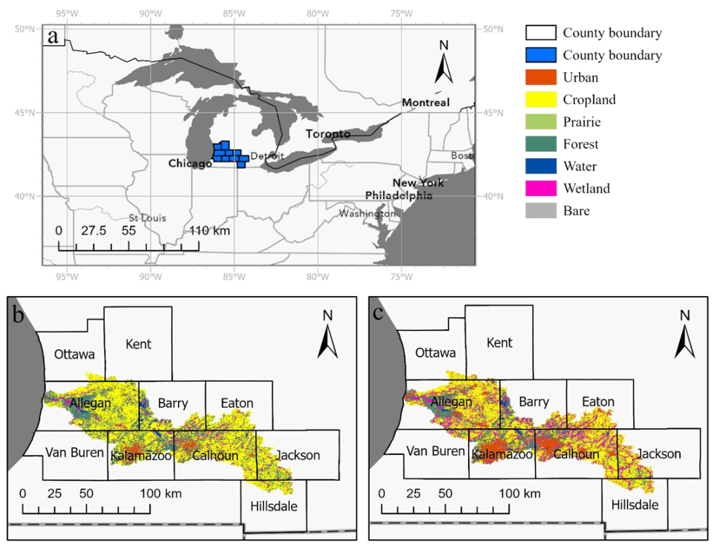
Fig. 1 The (a) Kalamazoo River Watershed in southwest Michigan with land cover in (b) 1986 and (c) 2017 presented for visual assessment of the change.

Next, we created a dataset of socioecological data and pulled from demographic, climate, soil and biophysical geospatial data (Table 1). This was exciting because all these resources come in different spatiotemporal resolutions, meaning that they’re estimated/collected at different rates and extents of time and space. They’re tricky to tie together because of this, so we needed to normalize them into intensity per unit area. Ultimately, we chose data that best represented our study site and our purposes, but there are many to choose from and this is not comprehensive list of what could be included.

Table 1 Variable, spatial extent (resolution), year, and data source used in the partial least squares structural equation model (PLS-SEM). 

Variable (unit for PLS-SEM)	Extent	Year	Source
POPD (population km-2), INC (income per capita km-2), UHD (housing unit km-2), RHD (rural housing unit km-2)	County	1980, 1990, 2000, 2010	Decadal Census, IPUMS (Ruggles et al., 2022)
FOR (% forest), WET (% wetland), BAR (% bare), CRO (% cropland), URB (% urban), WAT (% water), GRA (% grassland)	30 m	1986, 1991, 1996	Chen et al. (2019)
	30 m	2001, 2006, 2011, 2016	National Land Cover Database (Dewitz & Survey, 2021; Homer et al., 2020; Jin et al., 2019; Wickham et al., 2021; L. Yang et al., 2018)
IRR (% irrigation), NT (% no-till), CST (% conservation till km-2), CVT (% conventional till km-2), FD (count of farms km-2), FINC (net farm income km-2), FOW (% farmland owned km-2), FRF (% farmland rented from km-2), FRT (% farmland rented km-2), FLD (% farmland area per km-2), FINO (income per farm operation km-2)	County	1987, 1992, 1997, 2002, 2007, 2012, 2017	National Agricultural Statistic Service (NASS) (USDA National Agricultural Statistics Service, 2022)
NPP (net primary production kg C km-2)	30 m		Landsat CONUS (Robinson et al., 2018)
FP (farm phosphorus kg km-2), FN  (farm nitrogen kg km-2), NFP (non-farm phosphorus kg km-2), NFN (non-farm nitrogen kg km-2)	County		United States Geological Service (USGS) (Falcone, 2021)
PDI (Self-Calibrated Palmer Drought Severity Index)	4km		ScPDSI (Van der Schrier et al., 2013)
VPD (max vapor pressure deficit squared)	4 km		PRISM (Daly et al., 2008, 2015)
PTY (total annual precipitation mm), TPM (maximum air temperature standard deviation ˚C)	1 km		Daymet (Thornton et al., 1997)
GSL (annual growing season length, days)	4 km		This study
SPEI (standardized precipitation evapotranspiration index)			GRIDMET (Abatzoglou, 2013)
OMS (organic matter 0-5 cm km-2), SAS (sand 0-5 cm km-2), SIS (silt 0-5 cm km-2), PHS (average PH 0-5 cm km-2), CLS (average clay 0-5 cm km-2), OMD (organic matter 5-15 cm km-2), SAD (sand 5-15 cm km-2), SID (silt 5-15 mm km-2), PHD (average PH 5-15 mm km-2), CLD (average clay 5-15 mm km-2)	30 m		POLARIS (Chaney et al., 2016)
CRP (% Conservation Reserve Program county area enrolled)	County		USDA (FSA USDA, 2018)

Building a representative socioecological system model combined theory and statistics

We pulled from past work on human-nature interactions, sustainability, urbanization, and ecosystem responses to changing political landscapes.

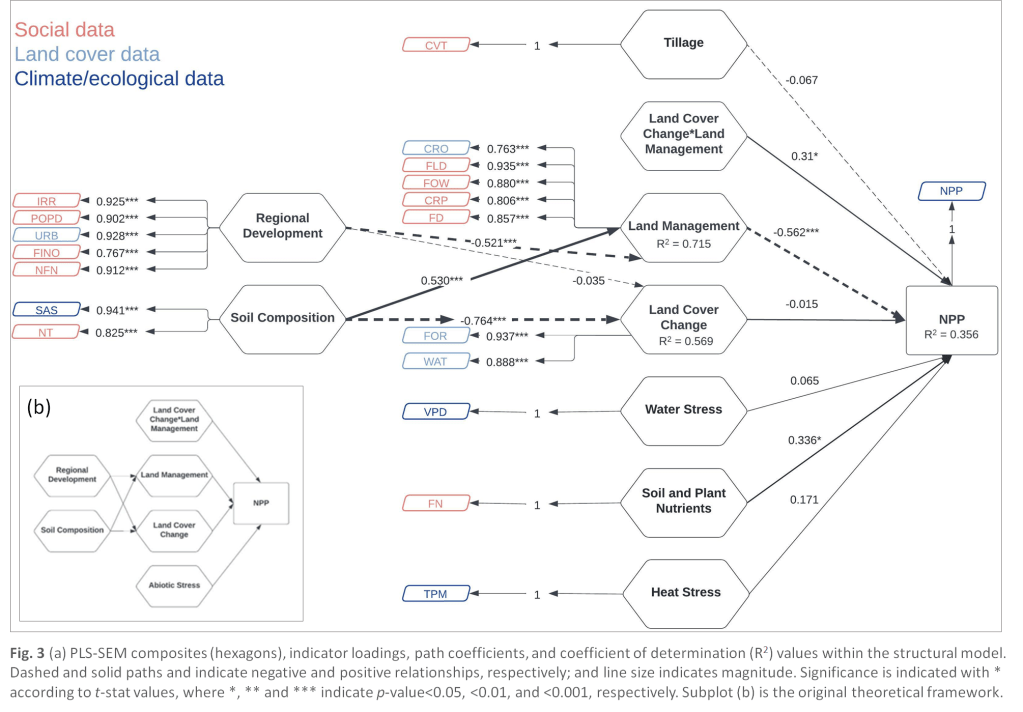
From these works, we built a theoretical framework to use (Fig 3b). In this framework, we hypothesize that net primary production (NPP, carbon production) is influenced by Land Management, Land Cover Change, and their interaction, as well as by Abiotic Stress. In addition, these are influenced by Regional Development and Soil Composition.

This framework is essential to building the partial least square structural equation model (PLS-SEM), where each of these categories are a ‘construct’ that will house our variables listed in Table 1.

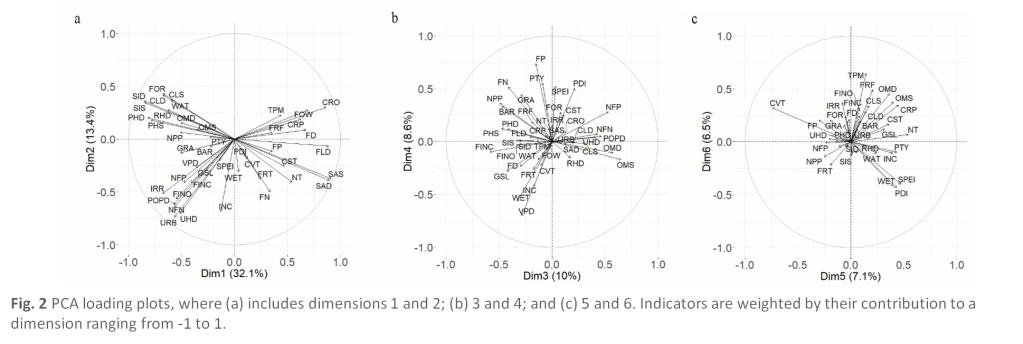
Next, we needed to figure out how to group our variables within these constructs. At this point, it can feel like a lot of guess work, so we turned to a principle component analysis (PCA). This way, we could allow all our variables in our dataset to be grouped statistically into similar dimensions and see how their collective variation explained the dataset’s variation. In a nutshell, it also helped me avoid bias when building constructs and ensure that my constructs had a better chance at ‘converging’ in the PLS-SEM.

The PCA indicated that ecological, climate and social data can each have strong relationships to a particular principal component or dimension (Fig 2). Therefore, a PLS-SEM composite could include a mix of socioecological variables.

The PLS-SEM underwent intermediary revisions, including removal of some indicators, before reaching convergence. New composites resulted from strong indicator loadings discovered in the PCA. If you’re curious about learning the stats and code behind building a PLS-SEM, I strongly recommend the “Partial Least Squares Structural Equation Modeling (PLS-SEM) Using R” workbook. It’s free and has numerous users, including a Facebook support group and a YouTube series mentioned in the text.

The PLS-SEM helped us evaluate the interactions between social, ecological and climate processes ‘everywhere’ and ‘all at once’… but without needing ‘everything‘.

The PLS-SEM underwent intermediary revisions, including removal of some indicators, before reaching convergence. New composites resulted from strong indicator loadings that we discovered in the PCA. Below is what the model’s final structure looked like (Fig 3a), with red, light blue, and dark blue noting social, land cover, and climate/ecological indicator data. You can also see how the composite ‘Abiotic Stress’ broke into other composites.

Does land cover change have a direct and significant effect on landscape NPP?

Yes. Cropland and forest structural composition and contribution to cumulative NPP hold the greatest influence on NPP 1987-2017, with little land cover change. In the composite ‘Land Cover Change’, forest (FOR) and water (WAT) performed best; whereas cropland (CRO) best performed with social data in the composite ‘Land Management’.  

Does regional development directly influence land management, and in turn shape the LCLUC and NPP of the landscape?

Yes. Regional Development, composed of social and land use data, has a significantly negative relationship with Land Management, which is composed of farmland data. This indicates that as Regional Development (e.g., urban area, irrigation, population density, etc.) increased, there is a decrease in Land Management (farmland and cropland, farmer-owned cropland, etc.). In turn, Regional Development has an insignificant, negative relationship with Land Cover Change (i.e., forest, water), likely due from little to no change in these land covers during the study period.

Do anthropogenic activities have a collectively higher and more influential direct impact on LCLUC than abiotic drivers?

Yes. Regional Development and Soil and Plant Nutrients had stronger relationships with NPP than abiotic processes Land Cover Change, Heat Stress or Water Stress. When Land Management interacted with Land Cover Change, there was a strong, positive relationship with NPP comparable to Soil and Plant Nutrients.

Did we model a bagel? Not really, hopefully our system is more simple than the multiverse!

I highly encourage anyone to explore PLS-SEM, especially landscape ecologists and geographers. You can use it when your dataset is small, non-normal, and missing data.

It’s a great way to advance your hypothesis/theory while you continue to collect more data. The sibling SEMs (CB-SEM, Bayesian SEM, Hierarchical SEM) also offer additional support once the dataset is robust enough.

Interested in reading more? This work is published in Landscape Ecology. Click here to view the article: rdcu.be/c9MHO

References

[1] Ruggles, S., Flood, S., Goeken, R., Schouweiler, M., & Sobek, M. (2022). IPUMS USA: Version 12.0 [dataset]. Minneapolis, MN: IPUMS. Retrieved from https://doi.org/10.18128/D010.V12.0.

[2] Chen, J., Sciusco, P., Ouyang, Z., Zhang, R., Henebry, G. M., John, R., & Roy, D. P. (2019). Linear downscaling from MODIS to Landsat: connecting landscape composition with ecosystem functions. Landscape Ecology, 34(12), 2917–2934. https://doi.org/10.1007/s10980-019-00928-2

[3] Dewitz, J., & Survey, U. S. G. (2021). National Land Cover Database (NLCD) 2019 Products (ver. 2.0, June 2021): U.S. Geological Survey data release. https://doi.org/10.5066/P9KZCM54

[4] Homer, C., Dewitz, J., Jin, S., Xian, G., Costello, C., Danielson, P., … Riitters, K. (2020). Conterminous United States land cover change patterns 2001–2016 from the 2016 National Land Cover Database. ISPRS Journal of Photogrammetry and Remote Sensing, 162, 184–199. https://doi.org/https://doi.org/10.1016/j.isprsjprs.2020.02.019

[5] Jin, S., Homer, C., Yang, L., Danielson, P., Dewitz, J., Li, C., … Howard, D. (2019). Overall methodology design for the United States National Land Cover Database 2016 products. Remote Sensing. https://doi.org/10.3390/rs11242971

[6] Wickham, J., Stehman, S. V, Sorenson, D. G., Gass, L., & Dewitz, J. A. (2021). Thematic accuracy assessment of the NLCD 2016 land cover for the conterminous United States. Remote Sensing of Environment, 257, 112357. https://doi.org/https://doi.org/10.1016/j.rse.2021.112357

[7] Yang, Limin, Jin, S., Danielson, P., Homer, C., Gass, L., Bender, S. M., … Xian, G. (2018). A new generation of the United States National Land Cover Database: requirements, research priorities, design, and implementation strategies. ISPRS Journal of Photogrammetry and Remote Sensing, 146, 108–123. https://doi.org/https://doi.org/10.1016/j.isprsjprs.2018.09.006

[8] USDA National Agricultural Statistics Service. (2022). Census of Agriculture. Retrieved from http://www.nass.usda.gov/Census of Agriculture/index.asp

[9] Robinson, N. P., Allred, B. W., Smith, W. K., Jones, M. O., Moreno, A., Erickson, T. A., … Running, S. W. (2018). Terrestrial primary production for the conterminous United States derived from Landsat 30 m and MODIS 250 m. Remote Sensing in Ecology and Conservation, 4(3), 264–280. https://doi.org/10.1002/rse2.74

[10] Falcone, J. A. (2021). Estimates of county-level nitrogen and phosphorus from fertilizer and manure from 1950 through 2017 in the conterminous United States. U.S. Geological Survey Open-File Report 2020–1153. https://doi.org/10.3133/ofr20201153

[11] Van der Schrier, G., Barichivich, J., Briffa, K., & Jones, P. (2013). A scPDSI‐based global data set of dry and wet spells for 1901-2009. Journal of Geophysical Research: Atmospheres, 118, 4025–4048. https://doi.org/10.1002/jgrd.50355

[12] Daly, C., Halbleib, M., Smith, J. I., Gibson, W. P., Doggett, M. K., Taylor, G. H., & Pasteris, P. P. (2008). Physiographically sensitive mapping of climatological temperature and precipitation across the conterminous United States. International Journal of Climatology, 28(15), 2031–2064. https://doi.org/10.1002/joc

[13] Daly, C., Smith, J. I., & Olson, K. V. (2015). Mapping atmospheric moisture climatologies across the conterminous United States. PLoS ONE, 10(10), e0141140. https://doi.org/10.1371/journal.pone.0141140

[14] Thornton, P. E., Running, S. W., & White, M. A. (1997). Generating surfaces of daily meteorological variables over large regions of complex terrain. Journal of Hydrology, 190, 214–251.

[15] Abatzoglou, J. T. (2013). Development of gridded surface meteorological data for ecological applications and modelling. International Journal of Climatology, 33(1), 121–131. https://doi.org/https://doi.org/10.1002/joc.3413

[16] Chaney, N. W., Wood, E. F., McBratney, A. B., Hempel, J. W., Nauman, T. W., Brungard, C. W., & Odgers, N. P. (2016). POLARIS: A 30-meter probabilistic soil series map of the contiguous United States. Geoderma, 274, 54–67. https://doi.org/10.1016/j.geoderma.2016.03.025

[17] FSA USDA. (2018). CRP enrollment and rental payments by county, 1986-2019. Retrieved from https://www.fsa.usda.gov/programs-and-services/conservation-programs/reports-and-statistics/conservation-reserve-program-statistics/index